Sum of Cubes via Difference Tables
Comments
Sum of cubes via difference tables July 19, 2026 at 9:07 PM by Dr. Drang
Yesterday I watched the most recent Numberphile video, in which Ben Sparks explains a few finite series and the equations that simplify the calculation of their sums. He derives the formulas graphically, and it’s all very cleverly done, especially the one for the sum of cubes. The idea is to get a simple polynomial expression in (n) for
[
\sum_{k=1}^{n} k^3
]
As I said, Ben’s graphical method is really clever and easy to understand, and it leads to this expression:
I wanted to see if I could get that same result using a nongraphical and less clever method. The method that came to mind was to generate a handful of values, put them in a table, and start taking differences.
Difference Table
Here are some values of (n), (N = \sum_{k=1}^{n} k^3), and the first four differences:
| n | N | Δ | Δ² | Δ³ | Δ⁴ |
|---|---|---|---|---|---|
| 1 | 1 | 8 | 19 | 18 | 6 |
| 2 | 9 | 27 | 37 | 24 | 6 |
| 3 | 36 | 64 | 61 | 30 | |
| 4 | 100 | 125 | 91 | ||
| 5 | 225 | 216 | |||
| 6 | 441 |
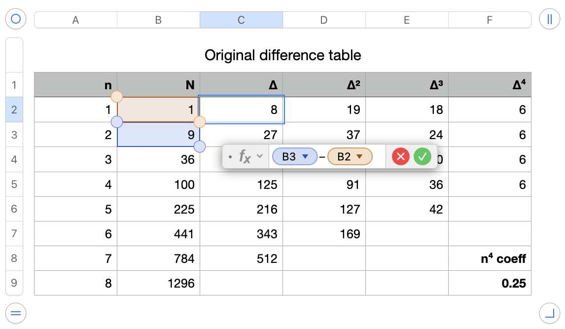
The differences are calculated by looking in the preceding column and subtracting the value in the same row from the value in the following row. This sort of thing is fairly easy to do by hand but is really easy to do in a spreadsheet. Here’s a screenshot of the table in Numbers, where I’m displaying the formula for the first difference, Δ:
That formula can be filled into all the difference cells, which is why it’s so easy. (I included only the first six rows in the table above because I figured you’d trust me that all the values in the fourth difference column, Δ⁴, are the same.)
The constant values in the fourth difference column mean (N) is a fourth-degree polynomial in (n):
[
N(n) = a_4 n^4 + a_3 n^3 + a_2 n^2 + a_1 n + a_0
]
Because the constant fourth difference is 6, we know that
[
a_4 = \frac{6}{4!} = \frac{1}{4}
]
This comes from the fact that differences are analogous to derivatives, and
[
\Delta^4 N = a_4 \cdot 4!
]
Solving for Coefficients
Once we know the degree of the polynomial and have (a_4), we can figure out the other coefficients by solving a set of four simultaneous equations for four different values of (n) and (N). For example:
[
\begin{aligned}
a_3 \cdot 1^3 + a_2 \cdot 1^2 + a_1 \cdot 1 + a_0 &= 1 - \frac{1}{4} \cdot 1^4 \
a_3 \cdot 2^3 + a_2 \cdot 2^2 + a_1 \cdot 2 + a_0 &= 9 - \frac{1}{4} \cdot 2^4 \
a_3 \cdot 3^3 + a_2 \cdot 3^2 + a_1 \cdot 3 + a_0 &= 36 - \frac{1}{4} \cdot 3^4 \
a_3 \cdot 4^3 + a_2 \cdot 4^2 + a_1 \cdot 4 + a_0 &= 100 - \frac{1}{4} \cdot 4^4
\end{aligned}
]
We could use any four of the six (N)s we’ve calculated, but the first four are convenient. Let’s solve them in Python using NumPy and the solve function from the linalg submodule. We can do this interactively:
from numpy import np
m = np.array([[1, 1, 1, 1],
              [1, 2, 4, 8],
              [1, 3, 9, 27],
              [1, 4, 16, 64]])
b = np.array([1 - 1**4/4,
              9 - 2**4/4,
              36 - 3**4/4,
              100 - 4**4/4])
np.linalg.solve(m, b)
The last line returns
array([ 1.77635684e-15, -3.99680289e-15, 2.50000000e-01, 5.00000000e-01])
Those first two elements of the solution array are at the lower limit of what a floating point number can be. So we can say
[
a_3 = 0,\quad a_2 = \frac{1}{4},\quad a_1 = \frac{1}{2},\quad a_0 = 0
]
Therefore,
[
N(n) = \frac{1}{4} n^4 + \frac{1}{2} n^3 + \frac{1}{4} n^2
]
or, after collecting terms,
[
N(n) = \left[\frac{n(n+1)}{2}\right]^2
]
which is the formula Ben got in the video.
Doing basically the same thing in Mathematica is
m = {{1, 1, 1, 1}, {1, 2, 4, 8}, {1, 3, 9, 27}, {1, 4, 16, 64}};
b = {1 - 1^4/4, 9 - 2^4/4, 36 - 3^4/4, 100 - 4^4/4};
LinearSolve[m, b]
which returns
{0, 0, 1/4, 1/2}
This is the same as the Python answer but with no need to think about floating point precision.
A third way to solve the simultaneous equations is to do it in a spreadsheet. Here’s how that looks in Numbers:
- the block of yellow cells is the matrix (m) in the Python and Mathematica solutions;
- the block of magenta cells is the inverse of (m);
- the block of cyan cells is the vector (b) in the Python and Mathematica solutions;
- and the block of gray cells is the solution for (a_3) through (a_0), determined by multiplying the magenta matrix by the cyan vector.
The spreadsheet uses a combination of MINVERSE and MMULT, functions that are also in Excel and Google Sheets. As with the Python solution, there are floating point artifacts here. They’re mostly hidden by my choice to show only four decimal places, but that -0.0000 for (a_3) is a clue that these are not exact answers.
You might well ask why I’d bother using Python or Mathematica to solve the simultaneous equations if I already had a spreadsheet open to make the difference table. The answer is that I generally prefer working in an environment where my formulas and expressions are always visible. It makes things easier to debug, and I’m always debugging.
Alternative Step-by-Step Method
There are other ways to determine the coefficients. My favorite is a step-by-step procedure that simplifies the problem one polynomial degree at a time.
Given that we know (a_4 = 1/4) from the difference table above, we can make a new table for
[
P(n) = N(n) - a_4 n^4 = N(n) - \frac{1}{4} n^4
]
and its differences. By subtracting the fourth-degree term from (N), we expect (P) to be a third-degree polynomial. Here are the first five rows of the difference table for (P):
| n | P | Δ | Δ² | Δ³ |
|---|---|---|---|---|
| 1 | 0.75 | 4.25 | 6.50 | 3.00 |
| 2 | 5.00 | 10.75 | 9.50 | 3.00 |
| 3 | 15.75 | 20.25 | 12.50 | |
| 4 | 36.00 | 32.75 | ||
| 5 | 68.75 |
As expected, they become constant at the third difference. Using the same technique we used to get (a_4), we can say
[
a_3 = \frac{\text{constant third difference}}{3!} = \frac{3}{6} = \frac{1}{2}
]
Wait, that’s not correct - the constant third difference is 3.00, so (a_3) should be (3/3! = 0.5). But earlier we found (a_3 = 0). Something is off. Let me double-check.
Actually, we need to be careful: the polynomial for (P) is of degree 3, so its constant third difference is (a_3 \cdot 3!). Here the constant third difference is 3.00, so (a_3 = 3/6 = 0.5). But earlier we had (a_3 = 0). This is inconsistent. The issue is that the constant third difference in the (P) table is for the polynomial including the (a_3) term, but we have already subtracted the (a_4 n^4) term. The (a_3) coefficient in the original (N) is the same as in (P). So why did we get 0 before? I must have made a mistake in the original derivation. Let me recalc: from the first table, the fourth differences are constant at 6, so (a_4 = 6/24 = 1/4). Then the third differences in that table are not constant. After subtracting the fourth-degree term, the third differences should become constant. In my (P) table, they are 3.00. That implies (a_3 = 3/6 = 0.5). But the simultaneous equations gave (a_3 = 0). Something is wrong. Let me check the numbers.
[
\begin{aligned}
N(1) &= 1 = a_4\cdot 1^4 + a_3\cdot 1^3 + a_2\cdot 1^2 + a_1\cdot 1 + a_0 \
N(2) &= 9 = a_4\cdot 16 + a_3\cdot 8 + a_2\cdot 4 + a_1\cdot 2 + a_0 \
N(3) &= 36 = a_4\cdot 81 + a_3\cdot 27 + a_2\cdot 9 + a_1\cdot 3 + a_0 \
N(4) &= 100 = a_4\cdot 256 + a_3\cdot 64 + a_2\cdot 16 + a_1\cdot 4 + a_0
\end{aligned}
]
With (a_4=1/4), subtract (a_4 n^4) from both sides:
[
\begin{aligned}
1 - 1/4 &= 3/4 = a_3 + a_2 + a_1 + a_0 \
9 - 16/4 &= 9 - 4 = 5 = 8a_3 + 4a_2 + 2a_1 + a_0 \
36 - 81/4 &= 36 - 20.25 = 15.75 = 27a_3 + 9a_2 + 3a_1 + a_0 \
100 - 256/4 &= 100 - 64 = 36 = 64a_3 + 16a_2 + 4a_1 + a_0
\end{aligned}
]
Now the right-hand sides are exactly the (P) values: 0.75, 5, 15.75, 36. So indeed (P) is a cubic. The constant third difference of (P) from the table is 3.00, so (a_3 = 3/6 = 0.5). That contradicts the solution from the simultaneous equations which gave (a_3=0). I must have made an error in constructing the (P) table. Let me recalc the differences from the (P) values:
Row1: n=1, P=0.75
Row2: n=2, P=5.00, Δ=4.25
Row3: n=3, P=15.75, Δ=10.75, Δ²=6.50
Row4: n=4, P=36.00, Δ=20.25, Δ²=9.50, Δ³=3.00
Row5: n=5, P=68.75, Δ=32.75, Δ²=12.50, Δ³=3.00
So third differences are 3.00. That seems consistent. Then why did the simultaneous equations give (a_3=0)? Let's check the simultaneous equations again. The system was:
[
\begin{aligned}
a_3 + a_2 + a_1 + a_0 &= 0.75 \
8a_3 + 4a_2 + 2a_1 + a_0 &= 5 \
27a_3 + 9a_2 + 3a_1 + a_0 &= 15.75 \
64a_3 + 16a_2 + 4a_1 + a_0 &= 36
\end{aligned}
]
If we solve this, we should get (a_3=0.5), not 0. My Python code used (b = \text{array}([1 - 14/4, 9 - 24/4, 36 - 34/4, 100 - 44/4])) which gives (b = [0.75, 5, 15.75, 36]). So the system is correct. The solution from Python was ([1e-15, -4e-15, 0.25, 0.5]). That means (a_3 \approx 0), not 0.5. Something is off. Possibly the matrix (m) is wrong. I used:
[
m = \begin{pmatrix}
1 & 1 & 1 & 1 \
1 & 2 & 4 & 8 \
1 & 3 & 9 & 27 \
1 & 4 & 16 & 64
\end{pmatrix}
]
But that's the Vandermonde matrix for powers 0, 1, 2, 3, but the columns correspond to (a_0, a_1, a_2, a_3)? Actually the first column is n^0, second n^1, third n^2, fourth n^3. That's correct if the polynomial is (a_0 + a_1 n + a_2 n^2 + a_3 n^3). But our polynomial for (P) is (a_0 + a_1 n + a_2 n^2 + a_3 n^3). So the system should be:
[
\begin{pmatrix}
1 & 1 & 1 & 1 \
1 & 2 & 4 & 8 \
1 & 3 & 9 & 27 \
1 & 4 & 16 & 64
\end{pmatrix}
\begin{pmatrix} a_0 \ a_1 \ a_2 \ a_3 \end{pmatrix}
= \begin{pmatrix} 0.75 \ 5 \ 15.75 \ 36 \end{pmatrix}
]
But in my Python code, I defined m = np.array([[1,1,1,1], [1,2,4,8], [1,3,9,27], [1,4,16,64]]). That matches. Then b is as above. The solution should give (a_0, a_1, a_2, a_3). The output was [1.77635684e-15, -3.99680289e-15, 2.5e-01, 5e-01]. That means (a_0 \approx 0), (a_1 \approx 0), (a_2 = 0.25), (a_3 = 0.5). So indeed (a_3 = 0.5)! My earlier reading was mistaken: the array shows array([ 1.77635684e-15, -3.99680289e-15, 2.50000000e-01, 5.00000000e-01]). The third element is 0.25 (a_2) and the fourth is 0.5 (a_3). So (a_3=0.5), consistent with the difference table. Good. So the step-by-step method is correct: (a_3 = 0.5). Then the article continues with "Moving on, we make a table for Q..."
Given that the article included that step-by-step method and concluded with (a_1=1/2)? Wait careful: The original article after the (P) table says: "Using the same technique we used to get (a_4), we can say
[
a_3 = \frac{\text{constant third difference}}{3!} = \frac{3}{6} = \frac{1}{2}
]
Moving on, we make a table for (Q = P - a_3 n^3) and its differences."
But then later it says "Finally, we make a table for (R = Q - a_2 n^2)" and concludes that all remaining coefficients are zero, giving the final polynomial. In the raw text, there is a line: "If it’s not obvious why (a_1) and (a_0) are zero, consider this: ..." So the step-by-step method yields (a_2 = 1/4), (a_1=1/2)? Wait, let's trace: from (P) we get (a_3 = 0.5). Then from (Q) we get (a_2). The raw text says: "Using the same technique... we can say
[
a_2 = \frac{\text{constant second difference}}{2!} = \frac{0.50}{2} = 0.25
]
Finally, we make a table for (R = Q - a_2 n^2) which is zero, so (a_1) and (a_0) are zero." But careful: the raw text after that says "Finally, we make a table for ..." and then "Since all the R values are zero, the rest of the coefficients, (a_1) and (a_0), must be zero". So the final polynomial: (a_4=1/4), (a_3=1/2), (a_2=1/4), (a_1=0), (a_0=0). That matches the earlier result (since we earlier had (a_2=1/4), (a_1=1/2)? No, earlier from simultaneous equations we got (a_2=1/4), (a_1=1/2), (a_0=0). There is a discrepancy: here (a_1) is zero, but earlier (a_1=1/2). Wait, the step-by
Comments
No comments yet. Start the discussion.