Dynamical System Transfer Learning with Reduced Order Models

Dynamical System Transfer Learning with Reduced Order Models Improving reinforcement learning for complex physics I have discussed previously the potential utility of applying Reinforcement Learning (RL) to analysis and control of complex physical systems. Developing RL algorithms to analyze or control complex dynamical systems faces one of the main challenges of many other RL problems - lengthy training times. This problem is complicated by the high computational cost of simulating complex physical dynamics. Compounding the thousands (perhaps millions) of RL training iterations needed for large state spaces and nonlinear systems with simulation times that may run into the hours (or even just minutes) per iteration can make problems intractable. Transfer learning has been used to reduce training times for RL problems and here we will explore application of transfer learning to RL for dynamical systems. Transfer learning relies on using models trained on similar problems to reduce training time with the assumption that the problem is similar enough that the model will have to make only small changes. For example, using an RL algorithm trained to drive a small RC car will probably more quickly learn how to drive a tractor trailer than one starting from scratch despite the considerable difference between the two. Reduced Order Models For physics simulations we need a problem environment to train the RL algorithm on that will be similar enough but substantially faster to simulate than the original. Reduced Order Models (ROMs) provide a way to generate such environments. A ROM, at its simplest, is a simplified model that seeks to reduce complexity while retaining as much accuracy as possible. There are many ways to generate ROMs. Any AI can be considered a ROM, from supervised learning to even large language models as ROMs of human language. Here we will apply unsupervised learning based on an approach outlined in Brunton and Kutz’s book Data Driven Science and Engineering to develop a data-driven ROM of a physical dynamical system based only on a data set of system measurements with little knowledge of the underlying system. As a brief introduction, dynamical systems are those that can be described as evolving through time. They are often summarized as where x is the state vector (set of variables that describe the system), dx/dt is the change in state with the change in time, and F(x) is some function of the state variables (sometimes including their history). The state vector x can be one variable or thousands, especially when state history is needed. F(x) may be a linear or nonlinear system. Linear systems have predictable response to input-double the input, double the response. Nonlinear systems, far more common and representative of the real world, do not exhibit that behavior throughout all possible states. Doubling input may double output, multiply output by 100, or drive output to 0, and this behavior can change depending on where you are in the state space (region of all possible values the variables can take). Real-world physical systems exhibit nonlinearity making them difficult to characterize. On top of that, realistic physical and engineering systems often lack solvable, direct, comprehensive governing equations that would support analysis of their behavior. The equations we can obtain, much less solve, often require simplification that constrict their utility to a subregion of the state space or lose track of higher order dynamics. Consider turbojet engine dynamics (which will be our example problem): the simulation we will use is based on a series of coupled equations that must be solved iteratively rather than directly solving a dynamic system of equations. Even then, it contains many simplifications of the coupled fluid, structural, thermodynamic, and chemical processes at work. Typical approaches, such as linearization around known solutions and creative use of coordinate systems, have become less helpful as complexity and scope of systems under analysis increase. However, as system complexity has exceeded traditional analytical approaches, our ability to gather, store, aggregate, and analyze measurement data at GB, TB, and even PB level has improved. Brunton and Kutz’s text discusses new techniques to approach dynamical systems exploiting increased measurement, storage, and analysis capabilities. Their approaches are based on unsupervised learning-that is looking for underlying patterns without a priori knowledge of what those patterns should be. These techniques use measurements of system state over time to derive dynamic models that can be used to describe, analyze, and predict behavior. The particular method we will use here is SINDy (Sparse Identification of Nonlinear Dynamics). Sparse Identification of Nonlinear Dynamics (SINDy) The goal of the SINDy algorithm is to discover system models in the form of mathematical equations using system measurement data, specifically a time series of state data that can be used to calculate an array of time derivatives of state variables over time. Essentially, it takes a candidate library of possible equation terms (such as products, quotients, and derivatives of states) and determines a parsimonious equation (that is, one that uses the fewest number of terms) that best describes the state changes over time. The basic equation describing SINDy is: where Θ(x) is the array of possible equation terms and Ξ is a matrix of coefficients for those terms. For example, if the equation exhibits strong quadratic behavior but no sinusoidal, then the value in Ξ corresponding to the quadratic vector of Θ(x) will have a large absolute value and the value corresponding to the sinusoid will be near 0. For more details, see the original SINDy paper: https://arxiv.org/abs/1509.03580 or a tutorial video:

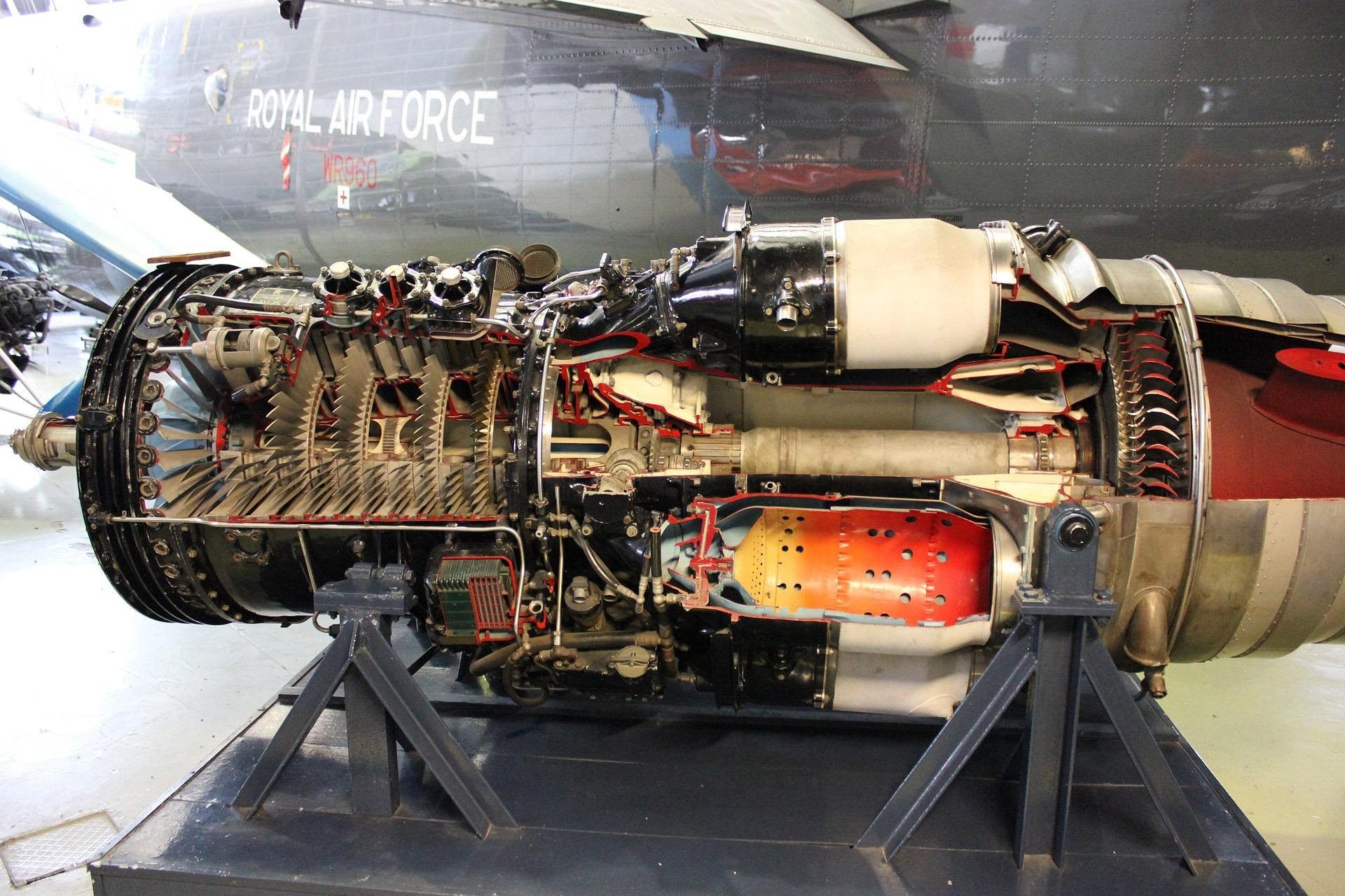
The SINDy algorithm has been able to identify complex fluid flow models just from time series data. Here we will see how well it can discover dynamic equations describing a turbojet engine (or at least describe the simulation we are using). Turbojet Modelling The specific problem here is creating an autothrottle for a turbojet engine. We want our RL algorithm to adjust the throttle on a turbojet engine to achieve a 10% change in speed at a given altitude, balancing time to new speed against fuel use. This is not a problem that would typically require reinforcement learning; autothrottle systems based on classical control, gain scheduling, or other techniques have been around for decades. Further, these other approaches have the advantage of being deterministic and so easier to certify for flight operations. Hence, I am not proposing this as a practical application of RL but chose it for convenience to illustrate the principles of (1) using RL on complex physical systems and (2) generating ROMs of complex physics as a source for transfer learning. Engines are the most complicated parts of an aircraft; generally speaking, the engine is about as hard to design as the rest of the aircraft. Solving for engine performance involves both aerodynamic and thermodynamic equations, both with rich and complex nonlinear behavior. I chose the turbojet problem specifically because of the complex physics and the availability of a reasonably high-fidelity model in Python. Turbojet engine operation is characterized by a balance of air and fuel mass flow, energy conservation, pressure ratios, non-constant gas dynamics, and other factors. Determining jet engine performance requires iteration-assume a set of gas properties such as density, pressure, temperature, velocity - at each of 6 or more stages through the engine, determine resulting mass flow and thermodynamics at each stage, and then iterate by adjusting assumptions for inlet mass flow, fuel flow, etc. until solution converges for particular operating parameters (speed in Mach number, altitude, and throttle setting). The Flight Test Engineering Github provides a jet engine simulator (along with an accompanying YouTube tutorial series) that allows definition of a jet engine and then simulation of its performance across a range of operating parameters. To account for variations in altitude and air compressibility, this simulation uses the ISA tools Python library which contains functions that translate altitude, temperature, density, speed, and Mach number based on the standard atmosphere. We will use this simulation as the foundation of a training environment for the baseline (non-transfer) RL algorithm and to provide the basis for a ROM. Even the “full” simulation used here is drastically simplified. Doing a full computational fluid dynamics model of even a small section of a jet engine takes tens of thousands of computational hours (and even that will contain substantial simplifications and assumptions about small-scale fluid dynamics and turbulence). Aircraft dynamics To match throttle setting to velocity change, we need to develop a basic aircraft model. We will use basic aerodynamics for a hypothetical aircraft that our engine will power. The RL algorithm will have to “learn” the drag behavior of this aircraft to properly set the throttle, with the drag in turn defined by aircraft aerodynamics. The aerodynamic parameters defining the aircraft and engine will be selected to provide realistic results. First, we define the engine. The turbojet simulator can design engine parameters such as compressor, combustor, and turbine given basic geometric parameters and a design point. We will define our engine around the performance of the J-47 used to power the B-47 Stratojet bomber. The B-47 had six engines, so we choose aerodynamic parameters at a scale of 1/6 of the B-47 and adjust from there for realistic performance, providing the following parameters m (mass) | 10000 kg | Cd0 (parasitic drag coefficient) | 0.0148 | AR (aspect ratio) | 5.0 | S (wetted surface area) | 22.2 m^2 | e (Oswald effic