Jacobian Conjecture for Baby

Comments

Jacobian Conjecture for Baby A step-by-step guide, starting from zero, to a famous math problem that stayed open for 87 years and then fell in July 2026. Every idea is shown as an animation, and you can check the final discovery yourself.

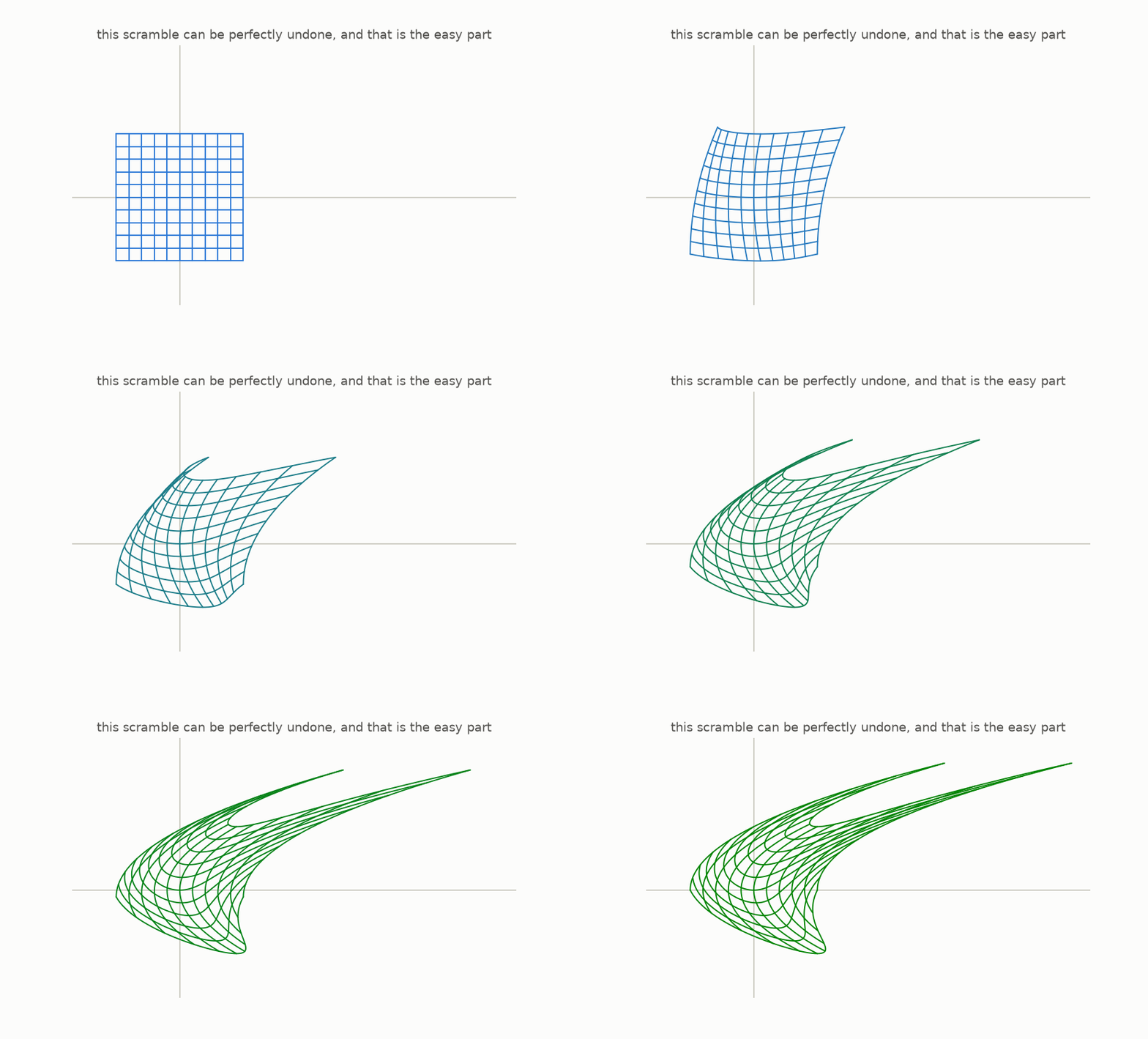
Look at this animation. A flat grid gets bent into a strange curved shape. It looks like the grid is ruined. It is not. This bending can be perfectly undone. There is a second simple rule that moves every point back to exactly where it started. Nothing is lost.

In 1939, a mathematician named Ott-Heinrich Keller asked a simple question about maps like this one. His question became one of the most famous unsolved problems in mathematics. Many mathematicians published proofs. Every proof turned out to be wrong. The problem stayed open for 87 years. Then, in July 2026, it fell. Only partly, and in a way nobody expected. (The original two-dimensional case is still open.)

This article explains the whole story from zero. You do not need any math background. Each chapter is one small idea, explained with a picture first. At the end, you can check the 2026 discovery with your own hands, using simple arithmetic. (Everything here is backed by an open repository: github.com/muchmirul/conjectures. It contains the code for every animation and a test suite that re-checks every mathematical claim.)

Here is the plan. Chapters 1 to 8 build the ideas one by one. Chapter 9 states the famous question. Chapters 10 to 12 tell what happened to it.

1 · Functions are machines

We start with the smallest idea: what a “function” is. A function is a machine. You feed it a number. It gives you back a number. That is all. The machine above uses the rule “double the number, then add 1.” Feed it 3, you get 7. Feed it 0, you get 1. Feed it 10, you get 21.

Two rules make a machine a function. First, it always gives an answer. Second, the same input always gives the same output, with no randomness and no “it depends”.

Now change the viewpoint. This new picture powers the rest of the article. Instead of feeding the machine one number at a time, imagine it moving every number on the number line at the same time. Same machine, new picture: a function moves the whole line. Keep this picture in mind. We will soon use it on bigger spaces.

One piece of notation, and it is the only one we need. Mathematicians name a machine with a letter like $f$ and write its rule as

$$
f(x) = 2x + 1.
$$

Read it as “$f$ takes a number $x$ and returns $2x + 1$.” The letter $x$ is just a placeholder for the input. The one thing to remember: a function is a machine that turns each input into exactly one output, and you can picture it moving every number at once.

2 · The undo machine

A machine moves every number. The next question is whether the move can be reversed. This small idea is the seed of the whole story.

The machine “double it” sends 3 to 6. The machine “halve it” sends 6 back to 3. Run one after the other, and every number ends up exactly where it started. When a second machine brings every output back to its original input, it is called the inverse, or the undo machine.

Doubling and halving undo each other. So do “add 5” and “subtract 5”.

Now try to undo “square it”, which multiplies the number by itself. Feed it −3: you get 9. Feed it 3: you also get 9. Now stand at 9 and try to walk back. Which input did you come from? You cannot know. The information “was it negative?” is gone.

An undo machine cannot exist when either of two things happens:

• Collisions: two different inputs land on the same output. (−3 and 3 both land on 9.)
• Gaps: some outputs are never produced, so the undo machine would have nothing to say there. (Squaring never outputs −4.)

If there are no collisions and no gaps, then every output has exactly one origin. So “walk back where you came from” is itself a machine. (The official words, if you want them: no collisions is called injective, no gaps is called surjective, both together is called invertible. You can forget these words. “No collisions, no gaps” is all you need.)

The one thing to remember: a machine can be undone exactly when no two inputs share an output and no output is missing. Undoing fails the moment information is destroyed.

3 · Polynomials

So far a machine could use any rule. The famous problem is about one specific family of machines: the ones built from nothing but plus and times.

Take an input $x$. Allow yourself only two operations, adding and multiplying, using numbers or pieces you have already built. Any machine you can build this way is called a polynomial.

• $2x + 1$ doubles and then adds one. It is a polynomial.
• $x^2$ is $x$ times $x$. It is a polynomial, since a power is just repeated multiplication.
• $x^3 - 2x$ builds $x \cdot x \cdot x$, builds $2x$, and subtracts. It is a polynomial, since subtracting is adding a negative.

Here are their graphs. For each input $x$ along the bottom, the height of the curve shows the output. The dashed gray curves, $\sin x$, $1/x$, and $\sqrt{x}$, are not polynomials. Each one needs an operation we did not allow: dividing by the input, or an infinite process.

Why focus on polynomials? Because they are the machines you can run exactly, with pencil and paper, in a finite number of steps. There is no approximation, no “undefined at zero”, and no infinite sums. They are the most concrete and most checkable machines in mathematics. That is what makes the coming problem so surprising. It is a question about the simplest machines we have, and it defeated everyone for 87 years.

One more word: the degree of a polynomial is its biggest power. So $x^3 - 2x$ has degree 3. This word becomes important in chapter 10.

The one thing to remember: a polynomial is any machine built using only plus and times. These are the most finite, most checkable machines there are.

4 · Maps of the plane

Machines that eat one number were the warm-up. Now our machines eat points. A point of the plane is a pair of numbers $(x, y)$: how far right, and how far up. A plane map is a machine that takes a point and returns a point.

A point is two numbers, so the machine has two output slots. Each slot may use both inputs:

$$
F(x, y) = (;\underbrace{\text{rule using } x, y}{\text{first slot}};,;; \underbrace{\text{rule using } x, y}{\text{second slot}};)
$$

In chapter 1, a machine moved the whole number line. A plane map moves the whole plane. To see it, draw a grid on the plane and watch the map carry it. The plane moves like a rubber sheet. The two dots are examples: each one is picked up at $(x, y)$ and put down at $F(x, y)$.

Here are six basic plane maps, all moving at once. Slide, turn, grow, and lean all keep the grid lines straight. The last one, bend, does not, because its rule uses $y^2$ and $x^2$, and squaring is what bends lines. This connects back to chapter 3.

A polynomial map of the plane is a map where both output rules are polynomials, built from $x$ and $y$ using only plus and times. For example, $F(x, y) = \left(x + \tfrac{1}{4}y^2,; y + \tfrac{1}{4}x^2\right)$ is the “bend” panel above. The rest of this article is about exactly these: polynomial maps of flat space.

The one thing to remember: a plane map moves every point of the plane at once, like a rubber sheet. It is a polynomial map when both of its rules use only plus and times.

5 · Straight maps and the area factor

Before we let maps bend anything, we need one number from the simplest maps. It is the most useful number in this story.

Some plane maps are perfectly regular. Grid lines stay straight, stay parallel, and stay evenly spaced, and the center point does not move. These are called linear maps, and we will call them straight maps. The turns, grows, squeezes, and leans of the last chapter are all straight maps.

Watch what each one does to the yellow square, which starts with area 1. There is a pattern here. A straight map scales the yellow square’s area by some factor, and it scales every piece of the plane, everywhere, by that same factor.

• turn, squeeze, and lean each give area × 1
• grow, which doubles everything, gives area × 4
• mirror gives area × 1, but the square comes out flipped, like a page turned over
• squash gives area × 0, and the whole plane lands on a single line

This one number, the area-scaling factor, is called the map’s determinant. For the mirror we record the flip with a minus sign, so its determinant is −1. The determinant therefore tells you two things at once: how much area is scaled, and whether the plane got flipped over.

Determinant zero is the disaster case. Watch the three dots. When the determinant is 0, the plane is pressed flat onto a line. Different points land on the same spot, which means collisions everywhere. Chapter 2 told us what that means: information destroyed, undo impossible.

And if the determinant is not zero? Then a straight map has no collisions and no gaps, and it has an undo map, which is also straight. For straight maps, one number decides everything: A straight map can be undone exactly when its determinant is not zero.

(Where the number comes from: a straight map is fully described by four numbers, $F(x, y) = (ax + by,; cx + dy)$. Its determinant is $ad - bc$. You will never need to compute this by hand here.)

The one thing to remember: a straight map scales all areas by one fixed factor, the determinant. If the factor is nonzero, the map can be undone. If the factor is zero, the plane is crushed and information is lost.

6 · Bending the grid

Now we let polynomial maps bend things, and we compare two kinds. Some maps bend the plane but never squeeze it. Others press area down to zero somewhere. This difference is the center of the whole story.

Start with the first kind. Here is the shear:

$$
F(x, y) = (x + y^2,; y)
$$

In words, it slides each horizontal row to the right by $y^2$. Rows near the middle barely move, and rows far away move a lot. Watch the yellow square as the plane bends. The grid bends, but nothing is squeezed or stretched, so every small piece keeps exactly its area.

This map is easy to undo. Each row slid right by $y^2$, so to undo it you slide it back:

$$
G(x, y) = (x - y^2,; y)
$$

$G$ undoes $F$ perfectly, and $G$ is itself a polynomial map. This is our first interesting polynomial map with a polynomial undo.

You can stack shears to build much wilder maps. Do a vertical shear, then a horizontal one. The two steps together form one polynomial map:

$$
H(x, y) = \left(,x + (y + x^2)^2,; y + x^2,\right)
$$

This is the bending from the very first animation of the article. It looks hopeless, but you know its secret: it is two simple shears, one after the other. To undo it, undo the layers in reverse order, like taking off your shoes and then your socks. Its undo map is again a polynomial, and in chapter 10 the computer will find it for us.

You can stack as many shears and straight maps as you like. The result looks more and more complicated, and it always stays perfectly undoable.

Now the second kind. Some polynomial maps destroy information. $F(x, y) = (x^2, y)$ folds the plane like closing a book, so the left half lands exactly on the right half. The two dots show a collision: two different points reach one landing spot. This map cannot be undone. $F(x, y) = (x, x\cdot y)$ crushes, so the entire vertical center line collapses onto one single point. It also cannot be undone.

Compare the two kinds. The shear and stacked shears bend but never crush, so they can be undone, with a polynomial undo. The fold and crush press area down to zero somewhere, which causes collisions, so they have no undo.

This looks like chapter 5’s rule, that a map can be undone exactly when its area factor is nonzero, trying to extend from straight maps to bent maps. But a bent map stretches area by different amounts in different places. So what plays the role of “the” area factor? For that we need a microscope.

The one thing to remember: stacked shears bend the plane into complicated shapes that are still easy to undo. Folds and crushes press area to zero somewhere, and they can never be undone.

7 · The microscope

Now the word that sounds the scariest in this subject: the Jacobian. It is just a microscope.

Take the curved graph of $y = x^2$ and zoom in on one point. Under the microscope, the curve straightens out. Zoom in enough and it looks exactly like a straight line. The slope of that line, here 2, is called the derivative at that point. This one observation, that smooth things look straight up close, is all the calculus you need today.

Now do the same with a bent grid. Take the stacked-shear map $H$ from the last chapter, pick the point $p = (0.5,, 0.5)$, and zoom in on what $H$ does near $p$. Straight. Parallel. Evenly spaced. This is exactly what chapter 5 described. Up close, a bent polynomial map looks just like a straight map.

The Jacobian of $F$ at a point $p$ is the straight map you see when you zoom in on $F$ near $p$. Different points show different straight maps under the microscope, so the Jacobian depends on where you look. (Computers find it by a mechanical rule, a small table of derivatives. You will never compute one by hand here; the computer does it in chapter 10.)

Here is why this matters. Straight maps have a determinant, an area factor. So at every point $p$, the map has a local area factor, written $\det J_F(p)$. It is the determinant of the straight map seen under the microscope at $p$. It says how strongly $F$ stretches or squeezes tiny pieces right at $p$, and whether it flips them.

Let us paint this number over the whole plane for two maps, and send a probe dot to read it out.

• The shear $(x + y^2, y)$ has local area factor exactly 1 at every point. At every location, under every zoom, it is a perfect area-preserving straight map. That is the precise meaning of “bends but never crushes”.
• The fold $(x^2, y)$ has local area factor $2x$. It is positive on the right half (blue), negative on the left half where that half got flipped (red), a